First, let us take a look at this grain size distribution curve.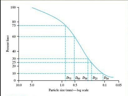

In this curve,

x axis – Particle size(dia) in mm in log scale

y axis – Percentage finer.

From this curve, we can find the D60, D30 and D10 of a particular soil.

D60 – 60 % of the soil particles are finer than this size.

D30 – 30% of the particles are finer than this size.

D10 – 10% of the particles are finer than this size.

Above definitions are just self explanatory. For example, if you have 100 particles of diameter ranging from 1 mm to 100 mm, D60 is 61 mm (below which 60% of particles are there).

Why do we find this?

To find Cu and Cc.

Cu – Uniformity coefficient.

Cu = D60/D10.

Cc – Coefficient of curvature.

Cc = (D30)^2 /(D60)(D10).

What is the use of this Cu and Cc?

Cu is always greater than 1 (equal to 1 is possible only by theoretical). If Cu is closer to 1 ( ie. D60 and D10 sizes are close to each other, which means there are more no. of particles are in the same size range), the soil is considered as uniformly graded.

If Cu is away from 1, the soil is well graded(ie. it has a vareity of size range distributed well). For gravel, if Cu>4, it is well graded. For sand, if Cu>6, it is well graded.

Cc is also greater than 1 ( equal to 1 is possible only by theoretical). For a well graded soil, Cc ranges between 1 to 3.

So,

Cu and Cc gives us idea about particle size distribution of a soil. These values are used in the soil classification.

Bonus points :

1. Why log scale is used instead of normal scale? If we use normal scale, it requires veryyyy length sheet to plot the soil size. Soil particles sizes ranges from few micrometers to centimeters range( 10^(-6) to 10^(-2) m ). So, it is impossible to cover this range with normal scale. Hence, log scale is used. And also getting a good curve is possible only with log scale.
2. For a uniformly graded soil, the grain distribution curve is almost vertical. For a well graded soil, the curve has a good slope. For a gap graded soil, the curve is almost horizontal in between any two points.